Tutorial: spherical Essential matrix and two-view triangulation

Field	Contract
Application	Estimate pose and sparse structure
Input	Two ERP images, or matched panorama-frame unit bearings
Output	Relative rotation, translation direction, and diagnostics
Strategy	Sphere-native bearing geometry
API	panorai.applications, panorai.features, panorai.estimators
Stability	Experimental
Dependencies	Core; feature frontend optional
Evidence	Executed analytic fixtures and documented failure cases

How this application is composed

SphericalRelativePose composes four typed stages: extract features from the ordered ERP pair, match them, convert the matches to panorama-frame bearings, then estimate the Essential matrix, rotation and unit translation direction. The final stage delegates to SphericalRelativePoseEstimator, so the wrapper does not duplicate the spherical epipolar residual, minimal hypotheses, robust consensus, local refinement or cheirality implementation.

Two central panoramas observe the same 3D scene from different centers. The previous tutorial produced matched unit bearings $(\mathbf b_1,\mathbf b_2)$. This tutorial turns them into relative rotation, translation direction, and arbitrary-scale 3D points.

See the Two-view geometry theme in the spherical computer-vision guide. Once features have become panorama-frame unit bearings, this tutorial uses no image convolution, gnomonic raster, or backprojection to ERP.

PanorAi-specific: five-bearing hypotheses, spherical tangent-Sampson scoring, panorama-frame pose conventions, cheirality selection and explicit quality/degeneracy diagnostics.

panorai.estimators is Experimental. It is useful research software with explicit diagnostics, not yet part of the Stable 3.x contract.

For an image-to-pose workflow, start with the application. Its default calls the frozen feature profile rather than manually recreating its component settings:

from panorai.applications import SphericalRelativePose

application = SphericalRelativePose()
pose = application(erp_1, erp_2)
if pose is None or not pose.quality_report.accepted:
    raise RuntimeError("relative pose was not trustworthy")

This profile includes the adaptive invalid-boundary guard and bilateral spherical match NMS. Bilateral here means duplicate suppression on both sets of bearings; it does not mean reciprocal FLANN cross_check, which remains disabled in the validated setup.

The same method can be inspected or adapted as an ordinary Pipeline:

from panorai.features import SphericalImagePair

pair = SphericalImagePair(erp_1, erp_2, "frame-1", "frame-2")
run = application.as_pipeline().run(
    pair,
    retain=("match_features", "bearing_correspondences"),
)
matches = run["match_features"]
correspondences = run["bearing_correspondences"]
pose = run.output

This is a sparse, non-differentiable geometry pipeline. It needs typed feature and estimator stages, all provided by PanorAi; it does not need a spherical convolution/pooling layer. Sphere-native raster ops and Torch layers remain available for learned or dense preprocessing before this pipeline, but are not silently inserted into the validated default.

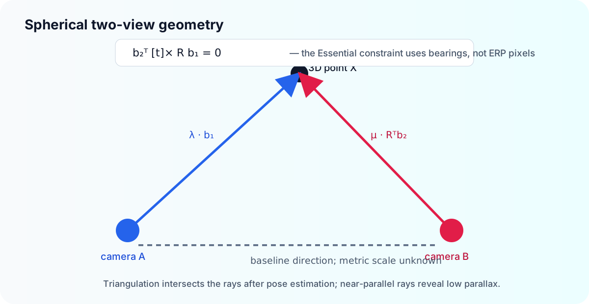
1. The spherical epipolar constraint

PanorAi defines relative pose by

$$ \mathbf x_2 = R_{21}\mathbf x_1 + \mathbf t_{21}. $$

For a correct correspondence, the two bearings and the baseline lie in one epipolar plane:

$$ \mathbf b_2^T E\mathbf b_1 = 0, \qquad E=[\mathbf t_{21}]\times R{21}. $$

The input is a pair of 3D unit bearings in the two panorama frames—not a pair of ERP pixels and not a mixture of pixels from different virtual cameras. This removes the planar camera matrix from the residual while retaining the same calibrated Essential geometry.

2. The five-point kernel used by PanorAi

Five calibrated bearing correspondences give five homogeneous linear equations in the nine entries of $E$. For correspondence $i$, PanorAi places

$$ \operatorname{vec}(\mathbf b_{2i}\mathbf b_{1i}^{T})^T $$

in row $i$ of a $5\times9$ design matrix $A$. In the generic case, $\operatorname{null}(A)$ has dimension four. If $E_1,\ldots,E_4$ are its basis matrices, every linear solution is

$$ E=x_1E_1+x_2E_2+x_3E_3+x_4E_4. $$

Most matrices in this nullspace are not Essential matrices. A calibrated Essential matrix must also satisfy the Demazure cubic constraints

$$ 2EE^TE-\operatorname{tr}(EE^T)E=0, \qquad \det(E)=0. $$

The implementation substitutes the four-dimensional nullspace into these nine matrix equations plus the determinant equation, giving ten cubic polynomials. For each of the four projective charts, one coefficient $x_k$ is fixed to one. The remaining three variables use the 20-monomial ordering of all terms up to degree three. Gaussian elimination expresses the ten cubic monomials through the ten-monomial quotient basis

$$ (x^2,xy,y^2,xz,yz,z^2,x,y,z,1). $$

Multiplication by $z$ in that quotient ring produces a $10\times10$ action matrix. Its real eigensolutions recover $(x,y,z)$ and therefore candidate Essential matrices. PanorAi tries all four charts so a valid solution whose chosen constant coefficient is zero is not silently discarded. Roots are checked against the original epipolar and calibrated-E constraints, normalized to unit Frobenius norm, and deduplicated up to the unavoidable $E\sim-E$ projective sign. If every polynomial chart is singular, a separately named deterministic nonlinear root search is used as a fallback.

FIVE_POINT(b1[1:5], b2[1:5]):
    A[i] <- vec(b2[i] b1[i]^T)^T
    N <- four-dimensional right nullspace of A
    candidates <- empty
    for constant coefficient k in {1,2,3,4}:
        substitute E = sum_j x[j] N[j], with x[k] = 1
        C <- coefficients of 9 Demazure cubics and det(E)
        if the cubic elimination block of C is well-conditioned:
            Mz <- 10x10 action matrix for multiplication by z
            for each real eigensolution of Mz:
                reconstruct E
                retain E only if the original constraints pass
                deduplicate E and -E
    if candidates is empty:
        run the declared numerical chart fallback
    return candidates

This is the calibrated five-point formulation introduced by Nistér (2004), implemented here with an explicit nullspace/action-matrix construction. See also Hartley and Zisserman, Multiple View Geometry, second edition and Szeliski, Computer Vision: Algorithms and Applications, second edition. The source implementation is panorai/estimators/_five_point.py.

Hartley image-point normalization is not applied at this stage. Its purpose is to condition homogeneous pixel coordinates in planar eight-point estimation. Here the inputs are already calibrated, unit-length 3D bearings. PanorAi instead validates bearing norms, distributes minimal samples over the sphere, checks the condition of $A$, tries four coefficient charts, and validates every root in the original equations.

3. Robust estimation around the minimal solver

The five-point kernel can return several algebraically valid roots, and any five matches can include an outlier. The complete estimator therefore wraps it in a spatially sampled, locally optimized robust loop:

SPHERICAL_RELATIVE_POSE(all bearing pairs):
    normalize valid bearings to unit length
    repeat the conservative RANSAC trial budget:
        draw five spatially diverse pairs without removing any scoring pair
        for E in FIVE_POINT(the five pairs):
            score tangent-Sampson residuals on every valid pair
            decompose E into (R1,+t), (R1,-t), (R2,+t), (R2,-t)
            choose the translation orientation using parallax-weighted cheirality
            form the provisional inlier set
            locally refine R and unit t with scale-marginal robust weights
            retain the best full-set hypothesis
    refine the winning consensus nonlinearly
    report residual, coverage, parallax, cheirality, stability,
        competing-model, and translation-orientation evidence
    return R and unit t; never claim translation scale

The nonlinear variables are three local rotation coordinates and two tangent coordinates on the unit sphere of translation directions. The objective is a robustly weighted signed spherical tangent-Sampson residual. It is a first-order epipolar objective rather than full two-view bundle adjustment; the quality report therefore remains part of the result contract.

3.1 Residual, robust score, and inlier update

For $q_i=\mathbf b_{2i}^{T}E\mathbf b_{1i}$ and the tangent projector $P_{\mathbf b}=I-\mathbf b\mathbf b^T$, the signed residual used by the optimizer is

$$ r_i(E)= \frac{q_i} {\sqrt{ \lVert P_{\mathbf b_{1i}}E^T\mathbf b_{2i}\rVert^2+ \lVert P_{\mathbf b_{2i}}E\mathbf b_{1i}\rVert^2 }}. $$

It is approximately an angular error in radians. A pair is provisionally consistent when $|r_i|\leq\tau$, where max_angular_error_deg supplies $\tau$. Cheirality is tested separately; the public inlier mask is the intersection of the residual test, explicit input validity, and positive depth under the selected pose.

PanorAi does not optimize a single hard-threshold count. For scales $s_k$ linearly distributed from scale_marginal_min_fraction * tau through $\tau$, it computes

$$ \omega_i= \frac{1}{K}\sum_{k=1}^{K} \left[\max!\left(1-\left(\frac{|r_i|}{s_k}\right)^2,0\right)\right]^2. $$

The default MSAC-first path orders hypotheses lexicographically by:

1. smaller normalized truncated-quadratic MSAC cost;

2. larger inlier count;

3. larger scale-marginal robust score;

4. smaller sum of inlier residuals.

Consequently, RANSAC selects a candidate using all available correspondences, not only the five rays that generated it. The dynamic trial bound is used only when the injected sampler satisfies the assumptions of uniform sampling.

hypothesis_ranking="msac-first" is the default and minimizes the normalized truncated-quadratic cost

$$ C_{\mathrm{MSAC}}(E)= \sum_i\min\left(\frac{r_i(E)^2}{\tau^2},1\right), $$

before using inlier count and the scale-marginal score as tie breakers. The "count-first" option preserves the former maximum-consensus ordering, and the scale-marginal-first variant promotes the existing continuous score ahead of hard inlier count. The estimator and these controls remain Experimental.

3.2 Optional all-inlier Essential refit

nonminimal_refit_max_steps optionally inserts the non-minimal counterpart of the normalized eight-point refit after a five-point consensus has been found. For the current inlier set $\mathcal I$, it constructs

$$ A_i=\operatorname{vec}(\mathbf b_{2i}\mathbf b_{1i}^{T})^T, \qquad i\in\mathcal I, $$

takes the last right singular vector of $A$ as a linear matrix estimate, and projects it onto the calibrated Essential manifold:

$$ E_0=U\operatorname{diag}(\sigma_1,\sigma_2,\sigma_3)V^T, \qquad E=U\operatorname{diag}(s,s,0)V^T, \qquad s=\frac{\sigma_1+\sigma_2}{2}. $$

The pose is rescored over every valid correspondence and the operation repeats until the inlier mask is unchanged, a previous mask recurs, the fit becomes rank deficient, or the configured cap is reached. The best hypothesis seen along the bounded trajectory is retained. Fewer than eight inliers skip this step. Hartley image-point recentering is not applied: the inputs are already calibrated unit bearings and affine translation of a spherical direction would change its geometry. The default cap is 100; the loop normally stops much earlier on a stable or repeated mask. Setting nonminimal_refit_max_steps=0 restores the former no-refit path. RelativePoseResult.consensus_refit_steps records the number of linear refits executed for the returned search path.

Real calibrated-pair guidance

For real feature correspondences with adequate support, the tested default is:

RelativePoseOptions()

The cap is deliberately loose: refitting stops earlier when the inlier mask stabilizes or cycles. A metadata-separated Hilti cam0 experiment froze predictions before opening the LiDAR-derived trajectory. In its 12-pair held-out phase, this combination reduced median oriented-translation error from 12.93 to 5.93 degrees, increased strict successes from 4 to 6, and reduced median rotation error from 1.01 to 0.90 degrees. The preregistered 25% rotation-reduction target was not met, so the API remains Experimental even though this is now the product default. Across both the development and held-out phases (30 pairs, descriptive only), median R/t errors fell from 0.785/8.396 to 0.398/5.933 degrees.

To reproduce the former compatibility behavior explicitly:

RelativePoseOptions(
    hypothesis_ranking="count-first",
    nonminimal_refit_max_steps=0,
)

One 33-match held-out pair returned no MSAC+refit pose, and translation was poorly observable for nearly stationary pairs. Always inspect quality_report.accepted; do not turn these observations into a universal match-count threshold. Full hashes, the OpenCV-to-PanorAi frame conversion, raw derived measurements and limitations are recorded under benchmarks/real_pair_relative_pose/.

3.3 Experimental decoupled rotation and translation

pose_refinement_method="decoupled" addresses a weak-parallax failure mode in which one Essential-matrix score selects an accurate rotation but an incorrect translation. It is opt-in; "joint" preserves the compatibility path.

The first stage estimates a rotation-only consensus from three-ray Wahba proposals,

$$ R^*=\arg\min_{R\in SO(3)}\sum_i |\mathbf b_{2i}-R\mathbf b_{1i}|^2, $$

and ranks proposals by truncated angular MSAC cost. Its threshold is $2.5\tau$, where $\tau$ is max_angular_error_deg. The inlier set is refit until stable, cyclic, or decoupled_refit_max_steps is reached. If fewer than half of the valid correspondences support a common rotation, the scene is not treated as far-background dominated and the estimator retains the joint pose.

For an applicable rotation, correspondences not explained by the rotation-only model form the translation pool. Each ray pair defines plane normals and a translation-axis proposal,

$$ \mathbf n_i=(R\mathbf b_{1i})\times\mathbf b_{2i}, \qquad \mathbf t_{ij}\propto\mathbf n_i\times\mathbf n_j. $$

Every proposal is evaluated over seven residual scales from $0.8\tau$ to $2.5\tau$. Support is accumulated only when the correspondence is epipolar, has positive-depth evidence, and has non-negligible parallax. Linear all-consensus refits use normalized plane normals and repeat to stabilization.

The selected direction must beat every candidate more than 10 degrees away by the relative score margin configured by decoupled_translation_min_score_margin (default 0.15). Fewer than five translation-pool rays are reported as unobservable; insufficient margin is reported as ambiguous. Both cases explicitly reject the two-stage result instead of presenting an unsupported translation as reliable.

RelativePoseResult.decoupled_pose_report records whether the method was applied, its rotation consensus, translation-pool and consensus sizes, score margin, iteration counts and fallback/abstention reason.

3.4 Nonlinear refinement of rotation and translation direction

Starting from $(R_0,\mathbf t_0)$, the optimizer uses a five-dimensional local parameter $\delta=(\delta\boldsymbol\omega,\delta\mathbf u)$:

$$ R(\delta)=\exp([\delta\boldsymbol\omega]\times)R_0, \qquad \mathbf t(\delta)= \frac{\mathbf t_0+B{\mathbf t_0}\delta\mathbf u} {\lVert\mathbf t_0+B_{\mathbf t_0}\delta\mathbf u\rVert}, $$

where the two columns of $B_{\mathbf t_0}$ span the tangent plane of the unit sphere at $\mathbf t_0$. Translation therefore retains unit norm and no metric scale variable is introduced. With robust weights frozen during one inner least-squares solve, the minimized objective is

$$ \min_{\delta\in\mathbb R^5} \sum_{i\in\mathcal I}\omega_i, r_i!\left([\mathbf t(\delta)]_\times R(\delta)\right)^2. $$

After an inner solve, the pose is rescored on the full valid set and accepted only if it improves the lexicographic rule above. Robust weights are then recomputed for the configured number of IRLS steps. Local optimization stops when a step does not improve the hypothesis or when local_optimization_steps is exhausted; one final refinement is attempted on the winning consensus. This is a bounded LO-RANSAC/IRLS procedure, not an unbounded nonlinear loop. When the optional non-minimal refit is enabled, its separate stabilization loop is bounded by nonminimal_refit_max_steps.

The optimizer’s internal SciPy scalar cost is not exposed as a public field. The inspectable result instead reports residual median/P90 and the normalized robust evidence under quality_report.model_competition.essential, together with inlier count, parallax, cheirality, stability, and rejection reasons.

4. Estimate relative pose

from panorai.estimators import RelativePoseOptions, SphericalRelativePoseEstimator

estimator = SphericalRelativePoseEstimator(
    RelativePoseOptions(
        max_angular_error_deg=0.5,
        random_seed=7,
    )
)
pose = estimator.estimate(matches.to_bearing_correspondences())
if pose is None or not pose.quality_report.accepted:
    raise RuntimeError("relative pose was not trustworthy")

R_21 = pose.R
t_21_direction = pose.t
inliers = pose.inlier_mask

The estimator builds five-correspondence Essential hypotheses, uses a spatially weighted but non-filtering RANSAC sampler, scores spherical tangent-Sampson error, refines rotation and translation direction, and selects the cheirally valid decomposition. The default orientation policy discounts depth signs supported only by nearly parallel rays; the historical raw-count policy remains available for reproducible A/B studies:

baseline_options = RelativePoseOptions(
    translation_orientation_method="positive-depth-count"
)
weighted_options = RelativePoseOptions(
    translation_orientation_method="parallax-weighted",
    translation_orientation_parallax_scale_deg=1.0,
)

A private C++ kernel may accelerate the same solver and residuals; Python retains policy, diagnostics, and fallback.

The CI-sized contract check is:

from panorai.estimators import RelativePoseOptions, SphericalRelativePoseEstimator

pose_estimator = SphericalRelativePoseEstimator(
    RelativePoseOptions(
        min_num_trials=8,
        max_num_trials=8,
        local_optimization_steps=0,
        minimal_solver_starts=8,
        minimal_solver_max_nfev=10,
        refinement_max_nfev=10,
        stability_trials=0,
        model_competition_trials=8,
        random_seed=7,
    )
)
pairwise_pose = pose_estimator.estimate(
    feature_matches.to_bearing_correspondences()
)
if pairwise_pose is not None:
    assert pairwise_pose.R.shape == (3, 3)
    assert pairwise_pose.t.shape == (3,)
    assert pairwise_pose.describe()["translation"] == "unit-direction-only"

Always inspect quality_report.accepted, rejection_reasons, angular coverage, residual percentiles, cheirality, parallax, stability, and competing rotation/projective models. A returned pose may intentionally carry a rejected quality report so experiments can audit it.

5. What is PanorAi and what is OpenCV here?

Stage	PanorAi route	OpenCV route
local features and descriptor neighbors	PanorAi façade, OpenCV implementation	SIFT, ORB, AKAZE, BFMatcher, FlannBasedMatcher
coordinates entering geometry	global panorama-frame unit bearings	normalized pinhole pixels/bearings chosen by caller
Essential hypothesis and robust policy	PanorAi five-point + spherical scoring	findEssentialMat for a calibrated planar-camera model
pose decomposition	PanorAi cheirality and quality report	recoverPose
public result	PanorAi RelativePoseResult + diagnostics	OpenCV arrays and masks

Both use calibrated Essential geometry. The PanorAi estimator is not a wrapper around cv2.findEssentialMat, and OpenCV feature extraction does not make the geometry itself OpenCV-owned. For the established planar APIs, consult OpenCV Camera Calibration and 3D Reconstruction. The feature backend does not alter the calibrated bearing equations above.

6. Resolve the orientation of translation

SVD of an Essential matrix produces two rotations and one translation axis, which means four pose hypotheses. Epipolar residuals cannot distinguish $t$ from $-t$ because $E$ and $-E$ describe the same epipolar planes. The missing orientation comes from triangulation and positive radial depth.

Concretely, after projecting $E$ to singular values $(s,s,0)$, let $E=U\operatorname{diag}(s,s,0)V^T$ and

$$ W=\begin{bmatrix}0&-1&0\1&0&0\0&0&1\end{bmatrix}. $$

The candidates are $R_1=UWV^T$, $R_2=UW^TV^T$, and $\mathbf t=\pm U_{:,3}$, with determinant corrections ensuring $R\in SO(3)$. The epipolar equation alone cannot choose among these four poses; the following cheirality evidence performs that selection.

The historical policy gave every correspondence one binary vote. That is fragile when $\theta_i$, the angle between the two triangulation rays, is close to zero: depth uncertainty grows approximately as $1/\sin\theta_i$, so tiny angular noise can reverse the depth sign of a distant point. The default policy now uses the bounded weight

$$ w_i=\frac{\sin^2\theta_i} {\sin^2\theta_i+\sin^2\theta_0}, \qquad \theta_0=1^\circ, $$

and selects the decomposition with the largest $\sum_i w_i,\mathbf1[\lambda_i>0\land\mu_i>0]$. Each reliable point is still capped at one vote, while an almost parallel pair contributes almost zero. If fewer than the five correspondences of a minimal calibrated solution reach $w_i\geq0.5$, PanorAi keeps the historical axis representative for compatibility but reports positive-depth-count-fallback, forces the orientation margin to zero, and therefore makes the quality policy abstain. translation_orientation records both weighted support and the historical raw counts, their separate margins, the scale $\theta_0$, and the selected method.

Weighting cannot create information. Pure rotation, uniformly distant scenes, or a baseline much smaller than scene depth must still be rejected through low parallax, competing rotation-only evidence, an ambiguous orientation margin, or unstable re-estimation. In those cases the axis ${t,-t}$ may be meaningful even when its orientation is not.

The reproducible comparison and raw samples live under benchmarks/translation_orientation/. It includes an isolated decomposition experiment and an end-to-end synthetic run on identical seeds. It is development evidence, not a replacement for a new outcome-blind VAL-002 real-image replay.

For an article-style, self-contained description of the estimator, see benchmarks/translation_orientation/ALGORITHM_PAPER.md. The numerical tables, environment, hashes, and measured comparison remain in results/TECHNICAL_REPORT.md.

7. Triangulate one inlier pair

Monocular relative pose observes only the direction of translation. PanorAi normalizes pose.t; choosing that unit baseline fixes an arbitrary scale. Camera B’s center in frame A is

$$ \mathbf C_2^{(1)}=-R_{21}^T\mathbf t_{21}, $$

and B’s bearing expressed in frame A is $\mathbf d_2^{(1)}=R_{21}^T\mathbf b_2$. Solve the closest points on

$$ \lambda\mathbf b_1 \quad\text{and}\quad \mathbf C_2^{(1)}+\mu\mathbf d_2^{(1)}, $$

then use their midpoint. Positive $\lambda$ and $\mu$ enforce cheirality; the angle between rays measures triangulation strength.

The following educational NumPy helper is executable, but is not a new public PanorAi API:

def triangulate_bearings(bearing_a, bearing_b, R_b_from_a, t_b_from_a):
    """Educational closest-rays triangulation in camera-A coordinates."""
    bearing_a = np.asarray(bearing_a, dtype=np.float64)
    bearing_b = np.asarray(bearing_b, dtype=np.float64)
    R_b_from_a = np.asarray(R_b_from_a, dtype=np.float64)
    t_b_from_a = np.asarray(t_b_from_a, dtype=np.float64)
    bearing_a /= np.linalg.norm(bearing_a)
    bearing_b /= np.linalg.norm(bearing_b)
    center_b_in_a = -R_b_from_a.T @ t_b_from_a
    ray_b_in_a = R_b_from_a.T @ bearing_b
    system = np.column_stack((bearing_a, -ray_b_in_a))
    depths, *_ = np.linalg.lstsq(system, center_b_in_a, rcond=None)
    point_on_a = depths[0] * bearing_a
    point_on_b = center_b_in_a + depths[1] * ray_b_in_a
    point_a = 0.5 * (point_on_a + point_on_b)
    ray_gap = float(np.linalg.norm(point_on_a - point_on_b))
    return point_a, depths, ray_gap

known_point_a = np.array([0.5, 0.2, 3.0])
known_center_b_a = np.array([1.0, 0.0, 0.0])
synthetic_R_ba = np.eye(3)
synthetic_t_ba = -known_center_b_a
synthetic_bearing_a = known_point_a / np.linalg.norm(known_point_a)
synthetic_bearing_b = known_point_a - known_center_b_a
synthetic_bearing_b /= np.linalg.norm(synthetic_bearing_b)
triangulated, depths, ray_gap = triangulate_bearings(
    synthetic_bearing_a,
    synthetic_bearing_b,
    synthetic_R_ba,
    synthetic_t_ba,
)
np.testing.assert_allclose(triangulated, known_point_a, atol=1e-12)
assert np.all(depths > 0.0) and ray_gap < 1e-12

For many correspondences, reject non-inliers first, then reject non-positive depth, very small ray angle, large closest-ray gap, or excessive angular reprojection error. Any recovered distance is expressed in the arbitrary unit baseline unless an external metric observation supplies scale.

8. Add the known tripod-height premise

Suppose the user records, for each photo, the distance from the camera’s optical center to one common, locally planar floor. Call those positive heights $h_A$ and $h_B$, in metres. A tripod-leg or tripod-head measurement must first be corrected by the fixed offset to the optical center.

We also need the floor-up unit vector $\mathbf g_A$ in camera A’s frame. It is [0, 1, 0] only when the ERP has been levelled to PanorAi’s +Y-up frame. Otherwise obtain it from an IMU, a trusted levelling step, or a separately estimated floor plane. The floor in camera A coordinates is

$$ \mathbf g_A^T\mathbf X_A+h_A=0. $$

This premise creates several different observability cases:

Available evidence	What becomes observable
spherical matches only	$R_{BA}$ and translation direction; structure has arbitrary scale
equal known heights, known up, no identified floor point	horizontal-baseline constraint and a useful consistency check; scale is still unknown
different known heights and known up	scale from the vertical baseline component, if that component is safely non-zero
at least one verified floor match plus a known height	metric baseline scale, including the common equal-height case
many floor matches or a floor mask	robust metric scale, metric floor points, and a plane-consistency diagnostic

The equal-height distinction is essential. If both centers are 1.60 m above the same floor, then their relative displacement has zero vertical component, but its horizontal length could still be 0.5 m, 2 m, or 20 m. Height alone does not choose between them.

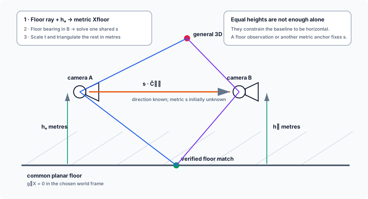
9. Intersect a floor ray in metres

For a bearing $\mathbf b_A$ known to hit the floor,

$$ \rho_A=-\frac{h_A}{\mathbf g_A^T\mathbf b_A}, \qquad \mathbf X_A=\rho_A\mathbf b_A. $$

The denominator must be negative. It approaches zero at the horizon, where a small angular error creates a very large range error; practical code therefore rejects a configurable horizon band. This operation already gives a metric 3D floor point from one levelled central panorama.

The uncertainty in $h_A$ transfers linearly into $\rho_A$. Uncertainty in the up vector and bearing grows nonlinearly near the horizon, so record the tripod measurement tolerance and do not present distant floor intersections as exact.

10. Recover the two-camera metric scale

Write PanorAi’s relative pose as

$$ \mathbf x_B=R_{BA}\mathbf x_A+s\widehat{\mathbf t}_{BA}, $$

where $\widehat{\mathbf t}_{BA}$ is the returned unit translation and $s>0$ is the unknown baseline length. For a verified floor correspondence, first compute its metric $\mathbf X_A$ from camera A’s height. Its prediction in B is

$$ \mathbf q_B+s\widehat{\mathbf t}{BA}, \qquad \mathbf q_B=R{BA}\mathbf X_A, $$

and must be parallel to the measured bearing $\mathbf b_B$. With $P_B=I-\mathbf b_B\mathbf b_B^T$, the one-dimensional least-squares solution is

$$ s=-\frac{(P_B\widehat{\mathbf t}{BA})^T(P_B\mathbf q_B)} {\lVert P_B\widehat{\mathbf t}{BA}\rVert^2}. $$

Use many spatially distributed floor matches, fit one shared positive $s$ with a robust loss, and report its dispersion. A match whose denominator is small does not constrain scale. Floor matches should establish scale after a relative pose supported by non-coplanar scene evidence; using only one plane to estimate the Essential geometry is a known degeneracy.

The executable educational implementation is intentionally not advertised as a public PanorAi API:

def intersect_floor(bearing, up_camera, camera_height_m, horizon_margin=1e-3):
    """Intersect one camera-frame unit bearing with its metric floor plane."""
    bearing = np.asarray(bearing, dtype=np.float64)
    up_camera = np.asarray(up_camera, dtype=np.float64)
    bearing /= np.linalg.norm(bearing)
    up_camera /= np.linalg.norm(up_camera)
    downward_component = float(up_camera @ bearing)
    if downward_component >= -horizon_margin:
        raise ValueError("bearing is above or too close to the floor horizon")
    radial_range_m = -float(camera_height_m) / downward_component
    return radial_range_m * bearing

def metric_scale_from_floor_match(
    floor_point_a, bearing_b, R_b_from_a, unit_t_b_from_a
):
    """Recover baseline scale from one verified floor correspondence."""
    bearing_b = np.asarray(bearing_b, dtype=np.float64)
    bearing_b /= np.linalg.norm(bearing_b)
    q_b = np.asarray(R_b_from_a, dtype=np.float64) @ floor_point_a
    unit_t = np.asarray(unit_t_b_from_a, dtype=np.float64)
    tangent_projector = np.eye(3) - np.outer(bearing_b, bearing_b)
    projected_t = tangent_projector @ unit_t
    denominator = float(projected_t @ projected_t)
    if denominator <= 1e-12:
        raise ValueError("floor match does not constrain translation scale")
    return -float(projected_t @ (tangent_projector @ q_b)) / denominator

up_a = np.array([0.0, 1.0, 0.0])
height_a_m = height_b_m = 1.60
center_b_a_m = np.array([1.20, 0.0, 0.35])
floor_point_a_m = np.array([2.0, -height_a_m, 4.0])
floor_bearing_a = floor_point_a_m / np.linalg.norm(floor_point_a_m)
floor_bearing_b = floor_point_a_m - center_b_a_m
floor_bearing_b /= np.linalg.norm(floor_bearing_b)
unit_t_ba = -center_b_a_m / np.linalg.norm(center_b_a_m)

metric_floor_point = intersect_floor(floor_bearing_a, up_a, height_a_m)
baseline_m = metric_scale_from_floor_match(
    metric_floor_point, floor_bearing_b, np.eye(3), unit_t_ba
)
metric_t_ba = baseline_m * unit_t_ba
recovered_center_b_a = -metric_t_ba

np.testing.assert_allclose(metric_floor_point, floor_point_a_m, atol=1e-12)
np.testing.assert_allclose(recovered_center_b_a, center_b_a_m, atol=1e-12)
assert np.isclose(up_a @ recovered_center_b_a, height_b_m - height_a_m)
# Equal known heights validate a horizontal baseline; without an observed
# floor point they do not determine the baseline length.

There is a second scale cue when $h_A\ne h_B$. Let $\widehat{\mathbf C}B^{(A)}=-R{BA}^T\widehat{\mathbf t}_{BA}$ be camera B’s center direction in A. Then

$$ s=\frac{h_B-h_A} {\mathbf g_A^T\widehat{\mathbf C}_B^{(A)}}. $$

This is ill-conditioned when the cameras are nearly at the same height, so the floor-correspondence estimate should remain the primary route for normal tripod captures. The height-difference equation is better used as an independent check or as evidence in a joint robust fit.

11. Recover scene structure in metres

After scale is accepted, replace the unit translation by $\mathbf t_{BA}^{metric}=s\widehat{\mathbf t}_{BA}$ and triangulate every non-floor inlier with the same closest-rays or angular-reprojection method. The resulting points and camera baseline are now in metres.

Use the geometry differently by point type:

• floor points: prefer direct ray-plane intersection; it uses the known metric plane and avoids unnecessary two-ray noise;

• general static points: triangulate with the scaled pose, then check positive depth, parallax, ray gap and angular reprojection in both cameras;

• object contact points: localize the contact on the floor, then use triangulated upper points to estimate metric object height;

• camera trajectory: camera B’s center in A is $-R_{BA}^T\mathbf t_{BA}^{metric}$; validate its vertical coordinate against $h_B-h_A$.

Do not silently convert all matches into floor constraints. Shadows, rugs, stairs, ramps, reflections, moving objects and incorrect semantic masks can produce a plausible but false scale.

12. Acceptance diagnostics for a metric result

A future metric helper should return a result only with diagnostics, including:

• the height, tolerance and optical-center offset used for each image;

• the up vector source and levelling residual;

• number and angular spread of candidate/accepted floor matches;

• per-match scale estimates, robust median, MAD and rejected outliers;

• minimum horizon margin and scale denominator;

• agreement between floor-derived scale and height-difference scale when both are conditioned;

• positive-depth rate, triangulation-angle distribution and angular reprojection percentiles for non-floor points;

• an explicit failure when the floor is not common/planar or metric scale is underconstrained.

This is the recommended route for evolving the library: first keep the closed-form example and synthetic oracle executable; then add an Experimental FloorPlanePrior/metric-scale result; only promote it after real captures with measured baselines and varied equal/different tripod heights.

13. Relation to standard two-view geometry

The derivation uses the calibrated Essential matrix, noisy-ray triangulation, and plane-induced homography results developed in Hartley and Zisserman, Multiple View Geometry in Computer Vision, second edition, sections 9.6, 12.1–12.3 and 13.1. For spherical cameras, ERP pixels are first converted to unit bearings, so the geometry already operates in calibrated normalized coordinates. The plane-induced bearing map is the same $H=R-\mathbf t\mathbf n^T/d$ relation, followed by direction normalization.

14. Two images are not yet a reconstruction system

Two-view triangulation cannot resolve weak parallax, repeated texture, dynamic objects, a misidentified floor, or metric scale without a valid external anchor. With three or more panoramas, tracks can corroborate points across views and global optimization can distribute error. Known heights can then be added as metric plane/center residuals instead of rescaling each pair independently. Continue to Tutorial: from matched panoramas to a multiview reconstruction.