Spherical region analysis¶

Region analysis turns masks or label fields into topology and geometry. A planar implementation is not sufficient for an ERP: its left and right edges are the same meridian, its pixels cover unequal solid angles, and a missing band must not connect regions merely because its numeric values are zero.

Each capability below is shown twice. The analytic figure isolates the mathematical contract; the real-image figure checks integration on the checksum-pinned CC0 Poly Haven Studio panorama. Its bright-region mask is a documented photometric heuristic, not semantic ground truth.

Read every real-image figure from left to right. The boxed line states the actual public call as input type → S.operation(...) → output type; numbered panels show those values; the final USE line states what that result enables in an application. The photograph is gamma-lightened for legibility only. All operations consume the original decoded values after the sphere-aware resize.

Topology contract¶

connected_components uses 4- or 8-neighbour ERP pixel-centre adjacency with periodic longitude. Latitude does not wrap. Unsupported or invalid pixels are absent vertices, so they cannot bridge components. Positive labels are deterministic and ordered by the first raster index of each component; zero is background.

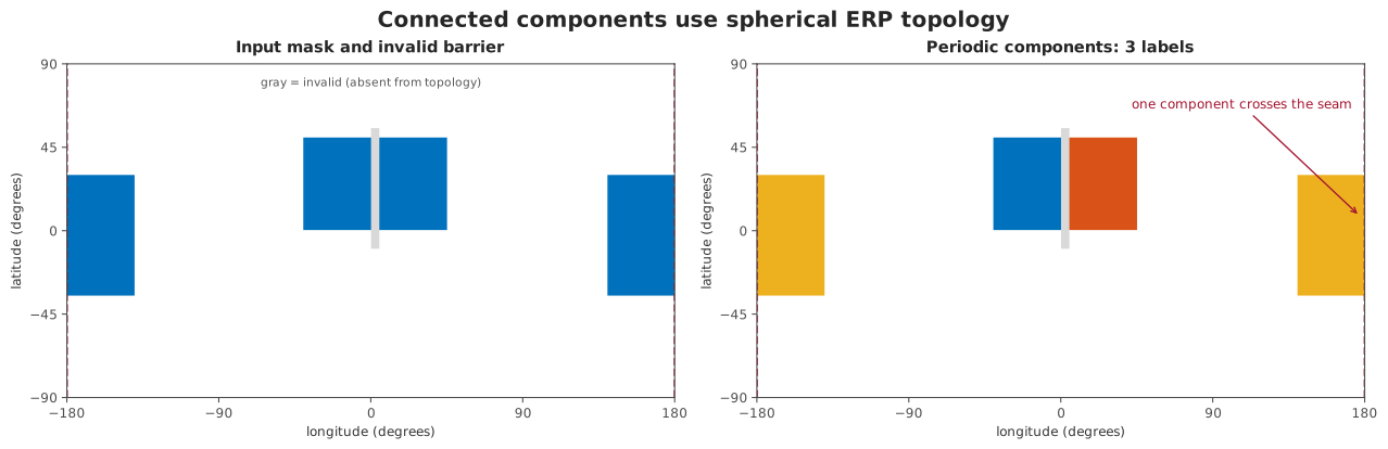
A seam-crossing ERP mask, an invalid barrier, and the resulting periodic connected-component labels. — Longitude is periodic, latitude is not, and invalid samples are absent from the topology. The seam-crossing blue region therefore receives one label; the gray barrier separates the central region.¶

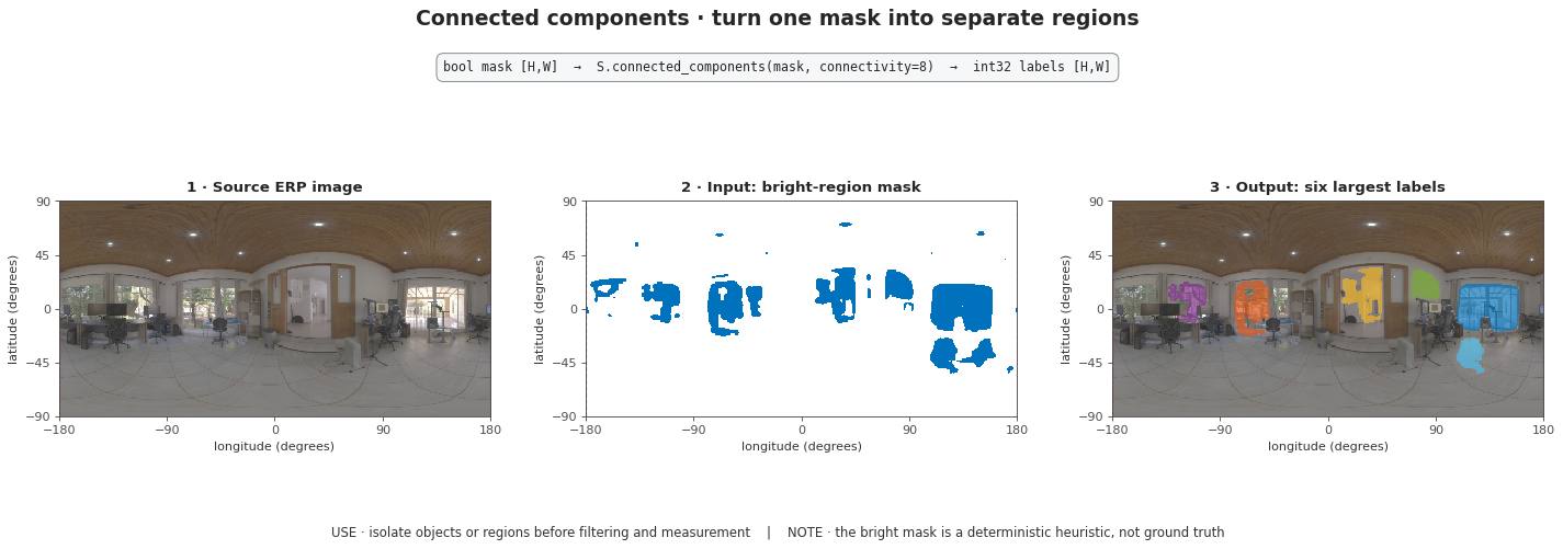
A real office ERP, its deterministic bright-region mask, and its six largest spherical connected components. — Real-image check. The source is loaded through `EquirectangularImage` and resized sphere-aware. The six largest components are selected by solid angle for display; the computation retains all 25 components. The bright openings and lamps make each retained region visually identifiable.¶

watershed floods the same graph from positive integer markers. It minimizes the maximum gradient along a path, then path length; the smaller marker label resolves a remaining tie. Marker pixels never change. This is a declared discrete graph watershed, not a planar watershed applied to an ERP rectangle.

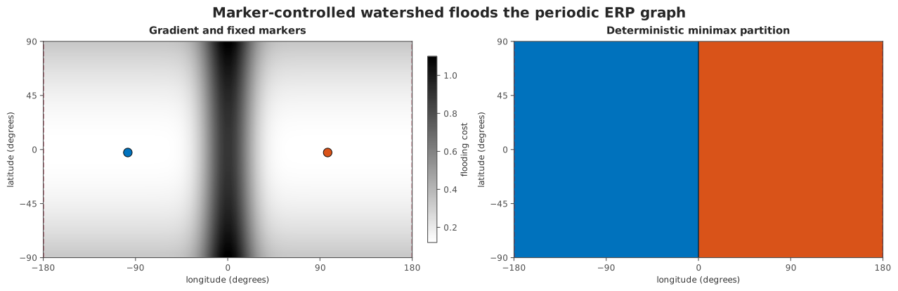
Two markers flooding an analytic ERP gradient into a deterministic spherical watershed partition. — Marker-controlled watershed operates on the same periodic graph. Fixed markers and deterministic tie-breaking make the partition reproducible.¶

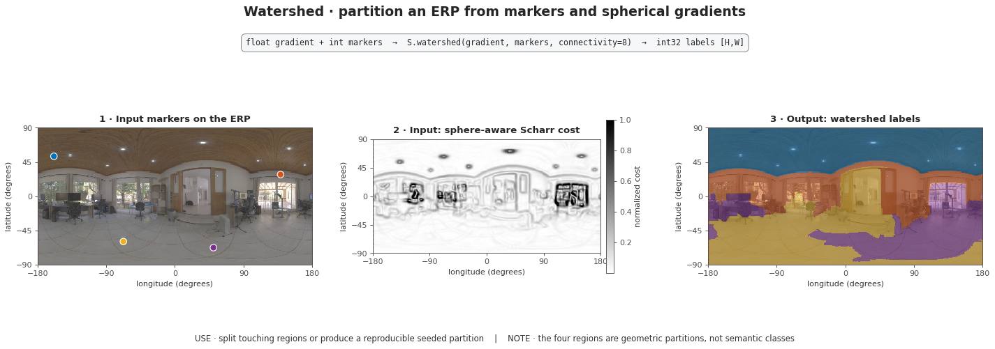
A real office panorama, its sphere-aware Scharr cost, four selected markers, and the resulting watershed regions. — Real-image check. Each marker is the lowest Scharr cost inside one of four fixed windows. The resulting regions follow real image ridges; they are geometric partitions, not semantic classes.¶

Distance and boundaries¶

geodesic_distance_transform builds unit bearings for ERP centres and returns the exact great-circle angle to the nearest selected centre. Values outside support or validity are NaN, not zero. region_boundaries uses topological neighbours and never invents a boundary at the longitude seam.

Angular perimeter is measured along cell interfaces. North-south interfaces have length \(\Delta\phi\); east-west interfaces at latitude \(\phi\) have length \(\cos(\phi)\Delta\lambda\). Solid angle comes from the existing spherical core and sums to \(4\pi\) over a complete ERP. Centroids are normalized solid-angle-weighted bearing sums. Symmetric regions whose vector sum is undefined return None rather than an arbitrary direction.

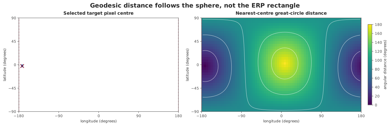
Equal colors mean equal angular distance on the sphere. They do not form Euclidean circles in the ERP rectangle, and the field remains continuous across the two displayed longitude edges.¶

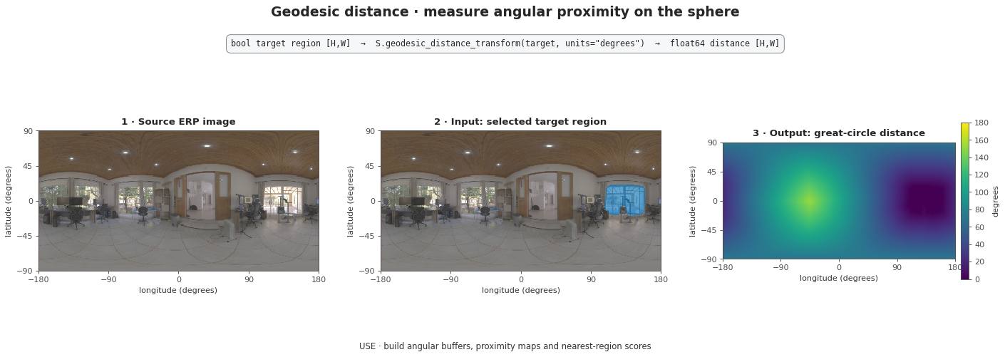
Great-circle distance from the largest bright region detected in a real office panorama. — Real-image check. Distance is evaluated from every ERP centre to the largest connected bright-region candidate and reported in degrees.¶

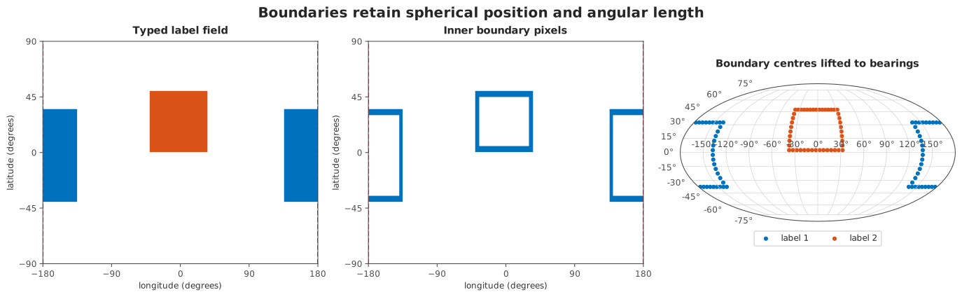
ERP labels, their inner boundary pixels, and the same boundary centres lifted to spherical bearings. — Raster boundaries can be retained as a typed mask or lifted to unit bearings. No artificial contour is introduced where the ERP is cut for display.¶

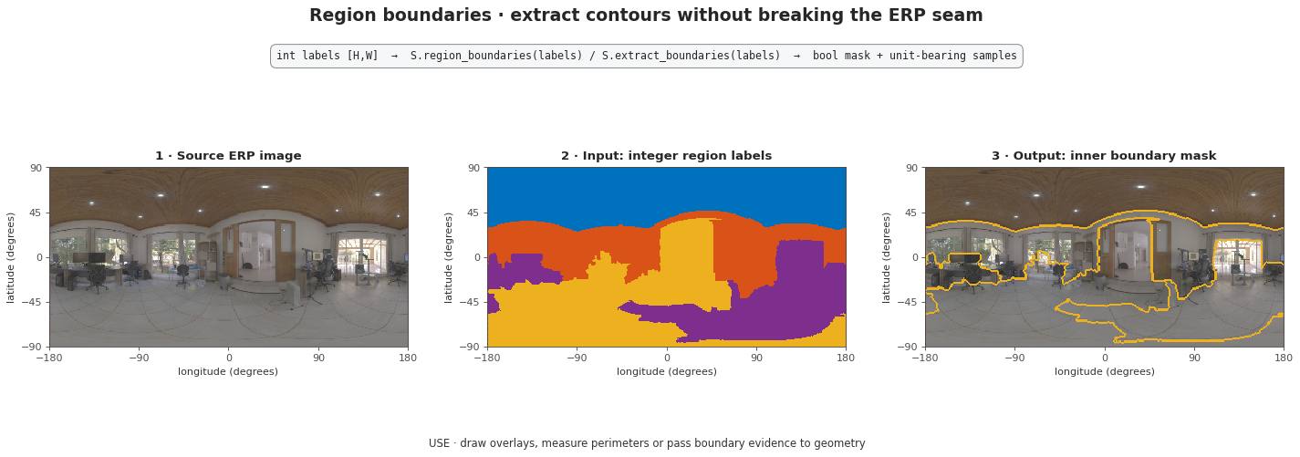
Watershed labels and their spherical inner boundaries over a real office panorama. — Real-image check. The yellow inner boundaries follow the real-image watershed and remain continuous at the longitude seam.¶

Ordered contours and medial axes¶

trace_contours follows ERP cell interfaces rather than sorting boundary pixel centres. Its vertices are therefore ordered, sub-pixel locations. The longitude seam is periodic and every cell corner on a polar edge is collapsed to the corresponding pole. A contour next to missing support or invalid data is open by default: closing it would assert a boundary that was never observed. Set include_support_boundary=True only when that explicit domain edge is the boundary an application intends to measure.

skeletonize returns a sampled spherical medial axis. It computes exact great-circle distance to the background at ERP pixel centres and retains intrinsic local ridges across opposite neighbour pairs. The result is a deterministic subset of the input mask, respects the longitude seam, never crosses invalid data, and can discard branches below a declared angular radius. This is not planar thinning applied to a wrapped rectangle. A mask filling its complete supported domain has no distinguished medial axis and fails explicitly.

Holes on a closed sphere¶

A sphere has no privileged exterior component. fill_holes therefore requires max_hole_solid_angle_sr. It fills only background components no larger than that physical area and never fills a component touching missing support or invalid data. The threshold is part of the scientific method, not an implementation detail.

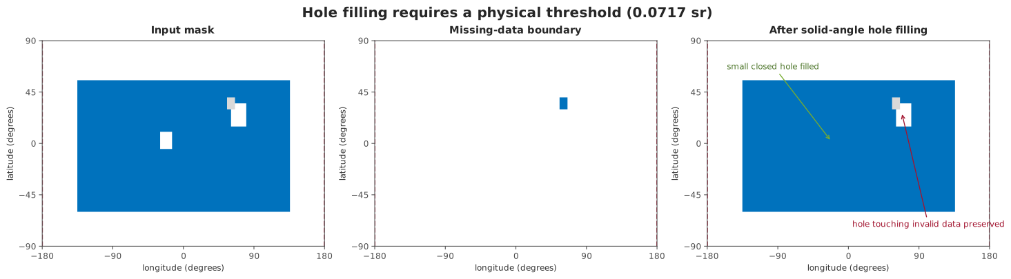
A small spherical hole filled by solid-angle threshold while a hole touching invalid data remains open. — The physical threshold fills the small closed component. A component that touches missing data remains unresolved instead of being silently treated as an interior hole.¶

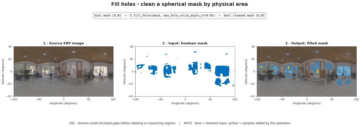
A real bright-region mask before and after solid-angle-constrained hole filling, with changed pixels highlighted. — Real-image check. Yellow samples are background components no larger than `0.05 sr` that were filled; blue samples were already selected by the photometric heuristic.¶

Measurements and adjacency¶

measure_regions and region_adjacency_graph expose complementary descriptions of a label field. Per-region values use spherical area, solid-angle-weighted centroids and angular perimeter. Graph edges store shared angular boundary length rather than a count of ERP pixels.

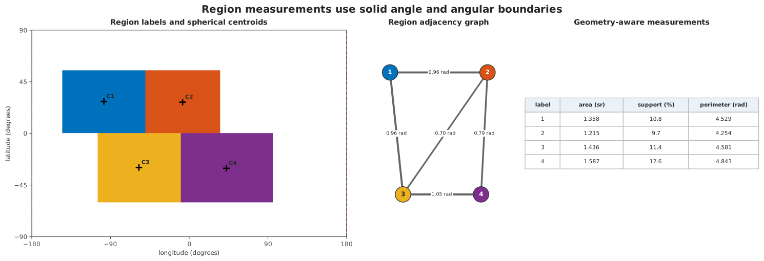
Four ERP regions with spherical centroids, their adjacency graph, and a table of physical measurements. — The raster, graph and table describe the same four regions. Measurements remain comparable across latitude because they are expressed in steradians and radians rather than raw pixel counts.¶

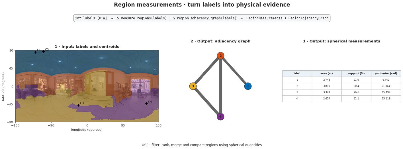
Real-image watershed regions with spherical centroids, adjacency graph, solid angle and angular perimeter. — Real-image check. The four partitions cover \(4\pi\); their centroid, area, perimeter and five adjacency edges are computed from spherical geometry rather than ERP pixel counts.¶

API placement¶

Functions and configured raster operations live in panorai.ops.spherical. Configured operations compose through EquirectangularImage.apply_spherical or OnSphere and safely persist in a Pipeline. SphericalWatershed is a two-field Stage; AnalyzeRegions turns a label field into RegionAnalysisResult. Immutable measurements, adjacency graphs, conservative enclosing caps, boundary samples and ordered contours live in panorai.data.

The Stable SphericalBoundary type intentionally stores unordered pixel-centre bearing samples. SphericalContour is the separate ordered cell-edge contract; neither is mislabeled as a filled spherical polygon.