Tutorial: spherical features and matching

Field	Contract
Application	Extract and match visual features
Input	One or two ERP images with optional validity masks
Output	Descriptors, ERP coordinates, unit bearings, and matches
Strategy	Projection-domain + spherical mapping; direct DoG is hybrid
API	SphericalFeaturePipeline
Stability	Stable face-based core; spherical DoG Experimental
Dependencies	Core OpenCV; PyCOLMAP optional
Evidence	Real CC0 output under a known longitude shift

How this application is composed

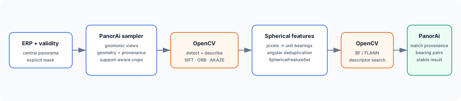
The face route composes projection, a planar OpenCV detector/descriptor, point-to-bearing lifting and angular NMS. The direct route composes spherical Gaussian convolution, resize and scale-space extrema from panorai.core, then uses tangent patches only for descriptors. SphericalFeaturePipeline is the recommended wrapper because it also preserves descriptor-row provenance, validity and matching defaults.

This tutorial extracts local features from an equirectangular panorama, expresses every keypoint as a panorama-frame unit bearing, and matches two panoramas without leaking OpenCV objects into the application.

The face-based extraction/matching core is Stable as panorai-spherical-features/v1. An additional direct spherical DoG detector is Experimental as panorai-spherical-dog-sift/v2. Both routes reuse OpenCV descriptors and nearest-neighbor search; PanorAi owns the sphere geometry, masks, deduplication, provenance, and public results.

See the Features and matching theme in the spherical computer-vision guide for the precise difference between Stable face-based detection, direct spherical DoG detection, descriptor-only tangent patches, and matching over descriptor arrays and bearings.

PanorAi-specific: virtual-camera geometry or direct spherical DoG, keypoint-to-bearing conversion, angular deduplication, masks and provenance. OpenCV still owns SIFT/ORB/AKAZE descriptors and BF/FLANN search.

The application card below uses the public CC0 Mosaic Tunnel ERP and a known 120° cyclic longitude shift. The plotted correspondences are real SphericalFeaturePipeline SIFT + FLANN matches; both halves retain the ERP seam so seam-adjacent evidence is auditable.

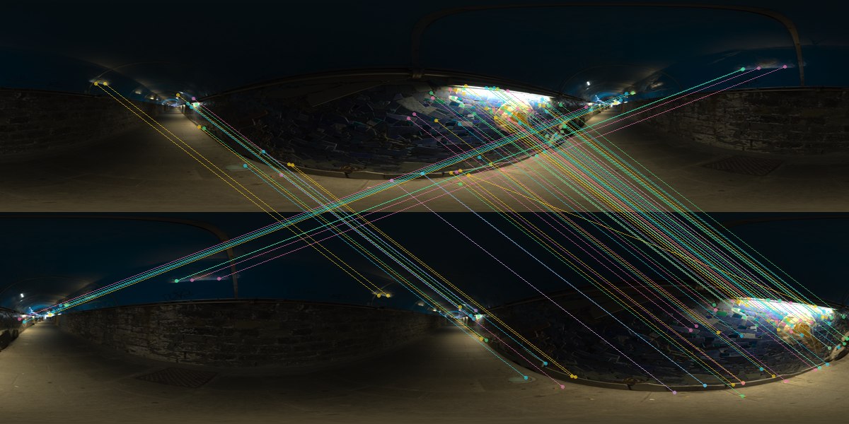
Exact source and derivative hashes, working resolution, and match counts are recorded in image provenance. The forest detector figures retained below are regression/generalization fixtures rather than the primary application scene.

If the input needs denoising or contrast normalization first, complete Tutorial: image processing on the sphere. Filtering the ERP with spherical neighbourhoods avoids introducing an artificial border before virtual-camera feature extraction.

1. Why not detect directly on the ERP?

An ERP stretches the poles and joins the left and right edges. A conventional planar detector sees that distortion and does not know the seam is periodic. PanorAi samples overlapping gnomonic views, lets OpenCV work on local pinhole rasters, maps keypoints back to unit rays, and removes overlap duplicates by angular distance.

2. Compare SIFT, ORB, and AKAZE

The figure below is generated by scripts/generate_documentation_figures.py from the CC0 panorama used in the previous tutorial. Each panel shows real features returned through PanorAi; color identifies the originating virtual face. The plotted subset is limited for readability, while the metadata records full counts.

Preset	Key idea	Descriptor / distance	Good starting point	Main trade-off
sift-flann	scale-space extrema and orientation-normalized gradients	float / L2, approximate FLANN	accuracy-first matching	slower and larger descriptors
sift-bf	same SIFT features, exhaustive matcher	float / L2, BF	smaller sets and deterministic search	exhaustive comparison cost
orb-hamming	FAST corners plus oriented BRIEF	binary / Hamming, BF	speed and compact storage	less scale/appearance tolerance
akaze-hamming	nonlinear scale space with binary MLDB	binary / Hamming, BF	a middle ground for textured scenes	thresholds remain scene-dependent

Technical background:

• SIFT: OpenCV tutorial and Lowe, 2004.

• ORB: OpenCV tutorial and Rublee et al., 2011.

• AKAZE: OpenCV tutorial and Alcantarilla et al., 2013.

No detector is universally best. Measure repeatability, match precision, runtime, and memory on the deployment domain.

3. Use the relative-pose reference profile

When the next operation is spherical Essential-matrix estimation, use the versioned reference profile instead of copying individual knobs:

pipeline = SphericalFeaturePipeline.for_relative_pose()
matches = pipeline.extract_and_match(
    erp_a,
    erp_b,
    panorama_id_a="capture-a",
    panorama_id_b="capture-b",
    validity_mask_a=valid_a,
    validity_mask_b=valid_b,
)

For a scanner with a missing south-polar cap, canonicalize the container before extraction. shadow_angle records the blind angle; shadow_padded says whether its rows already exist:

from panorai.data import EquirectangularImage

pano_a = EquirectangularImage(
    raw_a,
    shadow_angle=30.0,
    shadow_padded=False,  # cropped input; rows still need to be added
)
pano_a.preprocess()

pano_b = EquirectangularImage(
    raw_b_with_black_band,
    shadow_angle=30.0,
    shadow_padded=True,  # band already exists; do not add it again
)

matches = pipeline.extract_and_match(pano_a, pano_b)

The declared band becomes geometric non-support on every sampled face. Its RGB fill remains irrelevant: valid black structure outside the band is not masked. PanorAi refuses to project a positive shadow_angle while shadow_padded=False, preventing feature detection with the wrong vertical angle map. An explicit validity_mask can still describe additional sensor or application invalidity; it is separate from geometric support.

The v1 profile freezes six cube faces at 1024×1024 and 95° FOV, SIFT with a 4096-feature global cap, FLANN (trees=5, checks=50), Lowe ratio 0.72, 16-pixel face-edge exclusion, scale-aware validity exclusion at 1.5× keypoint scale, and 0.15° overlap/match deduplication. It also records preset_name="relative-pose-reference" in pipeline.describe().

The reference profile uses 4096×2048 ERPs with 1024-pixel/95° faces: a face should not ask for more average angular samples than the ERP contains. PanorAi does not silently resize the source, because the minimum useful resolution depends on scene detail, optics, and the accuracy target. Use the source resolution when it is higher, and run a resolution ablation for a new camera/domain before reducing it.

Pass real validity masks. Black pixels are not automatically invalid. The scale-aware guard rejects a keypoint when its descriptor footprint reaches invalid support, which prevents missing-data boundaries from forming a false consensus. CLAHE is not part of the reference profile.

This is a reproducible reference, not a universal optimum. Validate it on authorized Matterport3D and Stanford2D3D splits and always inspect the downstream pose quality report.

4. Select the minimum adequate resolution

for_relative_pose() deliberately freezes the validated operating point; it does not silently resize the ERP. When deployment cost requires a smaller raster, evaluate the same pair at an explicit increasing ladder and ask the Experimental selector whether the evidence has converged:

from panorai.features import (
    ResolutionSelectionObservation,
    ResolutionSelectionPolicy,
    select_feature_resolution,
)

# Application code evaluates each explicit ERP/face level and retains the
# real feature sets, matches, accepted pose result, and measured runtime.
observations = [
    ResolutionSelectionObservation(
        erp_shape_hw=level.erp_shape_hw,
        face_shape_hw=level.face_shape_hw,
        features_a=level.features_a,
        features_b=level.features_b,
        matches=level.matches,
        pose=level.pose,
        runtime_seconds=level.runtime_seconds,
    )
    for level in evaluated_levels
]
report = select_feature_resolution(
    observations,
    policy=ResolutionSelectionPolicy(target_rotation_accuracy_deg=0.15),
)
print(report.decision, report.selected_erp_shape_hw)

The selector compares mutual bearing repeatability, effective-inlier retention, spherical coverage and rotation change between adjacent levels. It chooses a lower level only when that transition and every remaining higher-resolution transition converge. Otherwise a usable highest level is reported as highest-resolution-fallback, with converged_plateau=False.

This report is Experimental. Its defaults are dataset-agnostic ratios and a caller-owned angular accuracy target, not a universal guarantee. Resolution levels must use the same masks, preprocessing policy, feature/matching profile and pose-quality policy; changing several variables at once invalidates the comparison. Translation-direction error should be inspected separately when ground truth is available.

5. Configure a general feature pipeline

from PIL import Image
import numpy as np
from panorai.features import SphericalFeaturePipeline

erp = np.asarray(Image.open("nature-reserve-forest-erp.jpg").convert("RGB"))
pipeline = SphericalFeaturePipeline.from_preset(
    "sift-flann",
    face_sampler="icosahedron",
    face_fov_deg=82.0,
    face_overlap_deg=8.0,
    face_shape_hw=(256, 256),
    edge_margin_px=8,
    max_features=700,
)
features = pipeline.extract(erp, panorama_id="forest-a")

print(features.describe())
print(features.source_erp_xy.shape, features.bearings.shape)

Each SphericalFeature retains its virtual-face pixel, optional ERP source pixel, unit bearing_xyz, response, scale, orientation, octave, descriptor row, projection specification, and duplicate provenance. Geometric support, input validity, an optional caller mask, and edge_margin_px are combined before OpenCV sees the image. Pixel color never determines validity.

The compact executable example used by CI is:

from panorai.features import SphericalFeaturePipeline

feature_height, feature_width = 128, 256
fy, fx = np.indices((feature_height, feature_width))
texture = (((fx // 9) + (fy // 11)) % 2 * 180).astype(np.uint8)
feature_rgb = np.stack(
    (texture, np.roll(texture, 5, axis=1), np.roll(texture, 7, axis=0)),
    axis=-1,
)
feature_pipeline = SphericalFeaturePipeline.from_preset(
    "sift-flann",
    face_sampler="cube",
    face_fov_deg=100.0,
    face_shape_hw=(96, 96),
    edge_margin_px=4,
    max_features=120,
)
feature_matches = feature_pipeline.extract_and_match(feature_rgb, feature_rgb)
assert len(feature_matches) > 0
assert feature_matches.bearings_a.shape[1] == 3
assert feature_pipeline.describe()["interface"] == "panorai-spherical-features/v1"

Optional contrast preprocessing

Solid-angle histogram equalization is useful to test when illumination leaves few repeatable keypoints. Apply the same preprocessing policy to both members of a matching pair and retain an unprocessed baseline; more contrast is not automatically better geometry.

from panorai.image_processing import spherical_equalize_histogram

enhanced_texture = spherical_equalize_histogram(texture)
enhanced_features = feature_pipeline.extract(
    enhanced_texture, panorama_id="equalized-frame"
)
assert enhanced_texture.dtype == np.uint8
assert len(enhanced_features) > 0

The real-image comparison and explanation of the latitude weighting are in Tutorial: image processing on the sphere.

6. Detect DoG extrema directly on the sphere

Use SphericalDoGSIFTPipeline when the detector itself must cross the ERP seam and retain one angular scale across latitude. Its Gaussian scale space uses spherical convolution; each 3D DoG extremum is compared with tangent neighbours on the sphere and receives an angular scale in degrees. There is no grid of overlapping virtual cameras and therefore no face-overlap duplicate to remove.

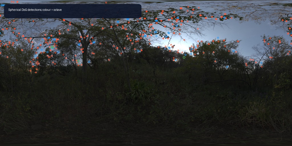
The descriptor is deliberately hybrid. PanorAi projects one small gnomonic patch centred on each accepted bearing, estimates a dominant tangent orientation, then calls cv2.SIFT.compute() at its centre. We do not reimplement the 128-value SIFT descriptor. Projection is local to description; it does not decide where keypoints exist.

from panorai.features import SphericalDoGSIFTConfig, SphericalDoGSIFTPipeline

dog_height, dog_width = 64, 128
dog_y, dog_x = np.indices((dog_height, dog_width))
dog_panorama = np.clip(
    128
    + 35
    * (
        np.sin(dog_x * 0.41) + np.sin(dog_y * 0.57) + np.sin((dog_x + dog_y) * 0.19)
    ),
    0,
    255,
).astype(np.uint8)
dog_pipeline = SphericalDoGSIFTPipeline(
    SphericalDoGSIFTConfig(
        octaves=2,
        max_features=100,
        contrast_threshold=0.003,
    )
)
dog_features = dog_pipeline.extract(dog_panorama, panorama_id="dog-a")
dog_shifted = np.roll(dog_panorama, 9, axis=1)
dog_shifted_features = dog_pipeline.extract(
    dog_shifted,
    panorama_id="dog-b",
)
dog_matches = dog_pipeline.match(dog_features, dog_shifted_features)
assert dog_features.descriptors.shape[1] == 128
assert dog_features.describe()["stability"] == "experimental"
assert len(dog_matches) > 0

The default descriptor is ordinary float SIFT with L2 matching. Set root_sift=True to L1-normalize and square-root each descriptor, while keeping the same L2 matcher. This API is Experimental: benchmark repeatability, match precision, runtime, and high-latitude behaviour before selecting it over the Stable face-based pipeline.

7. Match two panoramas

The example figure compares the panorama with a known 56-pixel cyclic longitude shift. This is a controlled seam demonstration, not an independent capture or an accuracy benchmark.

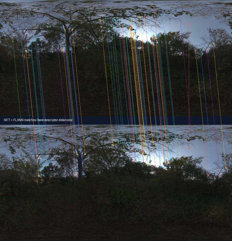
features_a = pipeline.extract(erp, panorama_id="forest-a")
features_b = pipeline.extract(np.roll(erp, 56, axis=1), panorama_id="forest-b")
matches = pipeline.match(features_a, features_b)

bearings = matches.to_bearing_correspondences()
assert bearings.bearings_a.shape == bearings.bearings_b.shape
assert bearings.bearings_a.shape[1] == 3

What the matcher parameters mean

• ratio_test: keep a nearest neighbor only when its distance is sufficiently smaller than the second-nearest distance. Lower is stricter. PanorAi presets use 0.75 for SIFT and 0.8 for binary descriptors.

• cross_check: require reciprocal descriptor assignments A→B and B→A. It can improve precision but reduces recall. It is off in the validated relative-pose profile; enabling it creates a different, unvalidated setup.

• max_distance: optional absolute cutoff in the descriptor’s own metric. L2 and Hamming distances are not comparable or calibrated probabilities.

• deduplicate_matches: applies bilateral spherical NMS after descriptor matching. A lower-distance match suppresses another only when their bearings are within the angular threshold in both panorama A and panorama B. This is on in the reference profile and is not cross_check.

• FLANN trees and checks: trade index/search work for approximate-neighbor quality. See the OpenCV FLANN guide.

Descriptor filtering is not geometric verification. A visually plausible match may still violate all physically possible camera motions. The next tutorial estimates a spherical Essential matrix from the aligned bearings.

8. Reproducibility checklist

Save pipeline.describe(), panorama IDs and checksums, feature/match describe() output, masks, and the chosen preset overrides. PanorAi does not turn descriptor distance into a universal confidence weight; the bearing correspondence adapter deliberately uses uniform valid weights.

Continue to Tutorial: spherical Essential matrix and two-view triangulation.